6. Taxonomic investigation
6.1. Preface
We want to investigate if there are sequences of other species in our collection of sequenced DNA pieces. We hope that most of them are from our species that we try to study, i.e. the DNA that we have extracted and amplified. This might be a way of quality control, e.g. have the samples been contaminated? Lets investigate if we find sequences from other species in our sequence set.
We will use the tool Kraken2 to assign taxonomic classifications to our sequence reads. Let us see if we can id some sequences from other species.
Note
You will encounter some To-do sections at times. Write the solutions and answers into a text-file.
6.2. Overview
The part of the workflow we will work on in this section can be viewed in Fig. 6.1.
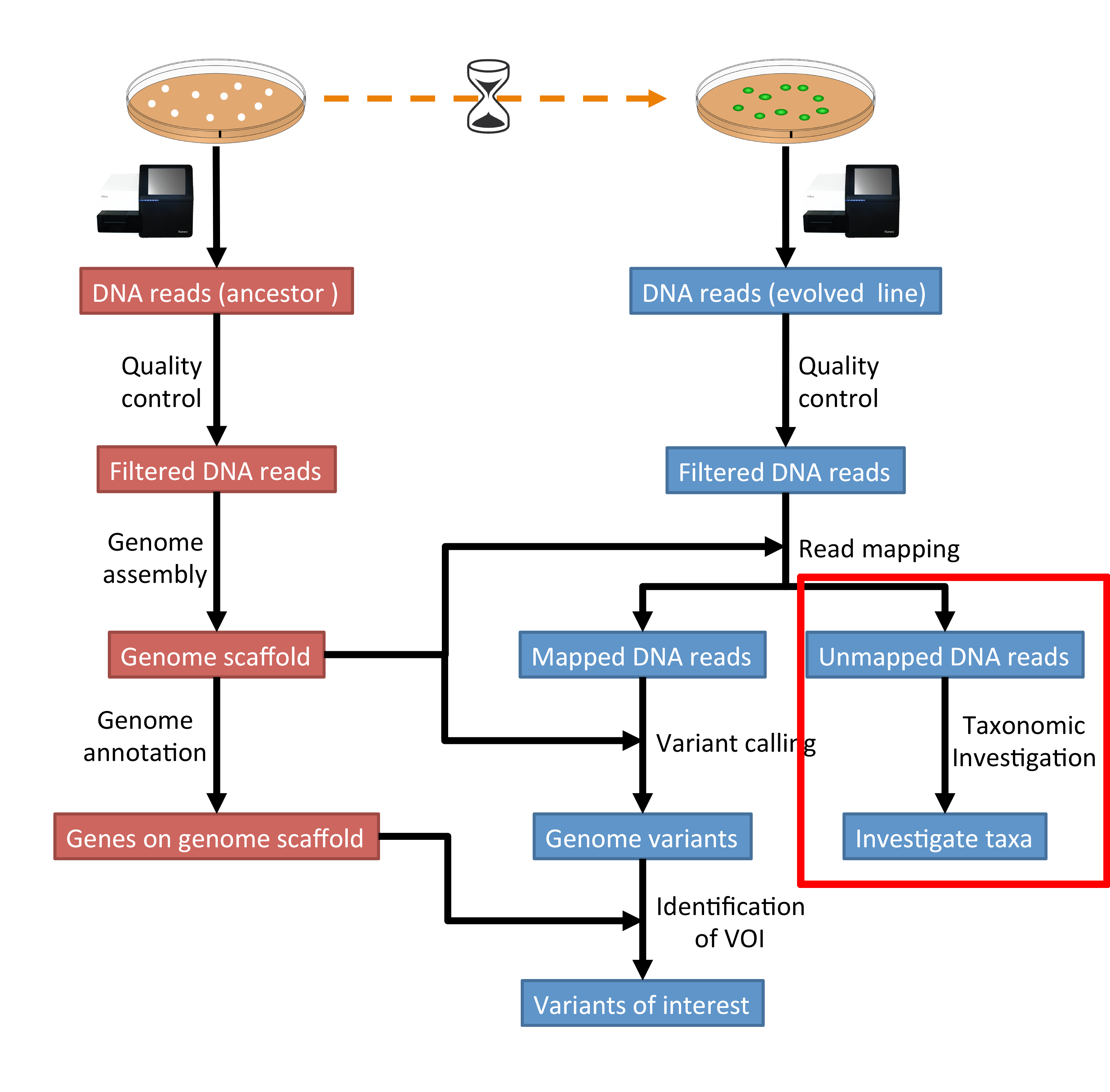
Fig. 6.1 The part of the workflow we will work on in this section marked in red.
6.3. Before we start
Lets see how our directory structure looks so far:
$ cd ~/analysis
$ ls -1F
assembly/
data/
mappings/
multiqc_data
trimmed/
trimmed-fastqc/
Attention
If you have not run the previous section Read mapping, you can download the unmapped sequencing data needed for this section here: Downloads. Download the file to the ~/analysis directory and decompress. Alternatively on the CLI try:
cd ~/analysis
wget -O mappings.tar.gz https://osf.io/g5at8/download
tar xvzf mappings.tar.gz
6.4. Kraken2
We will be using a tool called Kraken2 [WOOD2014]. This tool uses k-mers to assign a taxonomic labels in form of NCBI Taxonomy to the sequence (if possible). The taxonomic label is assigned based on similar k-mer content of the sequence in question to the k-mer content of reference genome sequence. The result is a classification of the sequence in question to the most likely taxonomic label. If the k-mer content is not similar to any genomic sequence in the database used, it will not assign any taxonomic label.
6.4.1. Installation
Use conda in the same fashion as before to install Kraken2. However, we are going to install kraken into its own environment:
$ conda create --yes -n kraken kraken2 bracken
$ conda activate kraken
Now we create a directory where we are going to do the analysis and we will change into that directory too.
# make sure you are in your analysis root folder
$ cd ~/analysis

# create dir
$ mkdir kraken
$ cd kraken
Now we need to create or download a Kraken2 database that can be used to assign the taxonomic labels to sequences. We opt for downloading the pre-build “minikraken2” database from the Kraken2 website:
$ curl -O ftp://ftp.ccb.jhu.edu/pub/data/kraken2_dbs/minikraken2_v2_8GB_201904_UPDATE.tgz

# alternatively we can use wget
$ wget ftp://ftp.ccb.jhu.edu/pub/data/kraken2_dbs/minikraken2_v2_8GB_201904_UPDATE.tgz

# once the download is finished, we need to extract the archive content:
$ tar -xvzf minikraken2_v2_8GB_201904_UPDATE.tgz
Attention
Should the download fail. Please find links to alternative locations on the Downloads page.
Note
The “minikraken2” database was created from bacteria, viral and archaea sequences. What are the implications for us when we are trying to classify our sequences?
6.4.2. Usage
Now that we have installed Kraken2 and downloaded and extracted the minikraken2 database, we can attempt to investigate the sequences we got back from the sequencing provider for other species as the one it should contain. We call the Kraken2 tool and specify the database and fasta-file with the sequences it should use. The general command structure looks like this:
$ kraken2 --use-names --threads 4 --db PATH_TO_DB_DIR --report example.report.txt example.fa > example.kraken
However, we may have fastq-files, so we need to use --fastq-input which tells Kraken2 that it is dealing with fastq-formated files.
The --gzip-compressed flag specifies tat te input-files are compressed.
In addition, we are dealing with paired-end data, which we can tell Kraken2 with the switch --paired.
Here, we are investigating one of the unmapped paired-end read files of the evolved line.
$ kraken2 --use-names --threads 4 --db minikraken2_v2_8GB_201904_UPDATE --fastq-input --report evol1 --gzip-compressed --paired ../mappings/evol1.sorted.unmapped.R1.fastq.gz ../mappings/evol1.sorted.unmapped.R2.fastq.gz > evol1.kraken
This classification may take a while, depending on how many sequences we are going to classify.
The resulting content of the file evol1.kraken looks similar to the following example:
C       7001326F:121:CBVVLANXX:1:1105:2240:12640        816     251     816:9 171549:5 816:5 171549:3 2:2 816:5 171549:4 816:34 171549:8 816:4 171549:2 816:10 A:35 816:10 171549:2 816:4 171549:8 816:34 171549:4 816:5 2:2 171549:3 816:5 171549:5 816:9
C       7001326F:121:CBVVLANXX:1:1105:3487:12536        1339337 202     1339337:67 A:35 1339337:66
U       7001326F:121:CBVVLANXX:1:1105:5188:12504        0       251     0:91 A:35 0:91
U       7001326F:121:CBVVLANXX:1:1105:11030:12689       0       251     0:91 A:35 0:91
U       7001326F:121:CBVVLANXX:1:1105:7157:12806        0       206     0:69 A:35 0:68
Each sequence classified by Kraken2 results in a single line of output. Output lines contain five tab-delimited fields; from left to right, they are:
C/U: one letter code indicating that the sequence was either classified or unclassified.The sequence ID, obtained from the FASTA/FASTQ header.
The taxonomy ID Kraken2 used to label the sequence; this is 0 if the sequence is unclassified and otherwise should be the NCBI Taxonomy identifier.
The length of the sequence in bp.
A space-delimited list indicating the lowest common ancestor (in the taxonomic tree) mapping of each k-mer in the sequence. For example,
562:13 561:4 A:31 0:1 562:3would indicate that:the first 13 k-mers mapped to taxonomy ID #562
the next 4 k-mers mapped to taxonomy ID #561
the next 31 k-mers contained an ambiguous nucleotide
the next k-mer was not in the database
the last 3 k-mers mapped to taxonomy ID #562
6.4.3. Investigate taxa
We can use the webpage NCBI TaxIdentifier to quickly get the names to the taxonomy identifier. However, this is impractical as we are dealing potentially with many sequences. Kraken2 has some scripts that help us understand our results better.
Because we used the Kraken2 switch --report FILE, we have got also a sample-wide report of all taxa found.
This is much better to get an overview what was found.
The first few lines of an example report are shown below.
83.56  514312  514312  U       0       unclassified
16.44  101180  0       R       1       root
16.44  101180  0       R1      131567    cellular organisms
16.44  101180  2775    D       2           Bacteria
13.99  86114   1       D1      1783270       FCB group
13.99  86112   0       D2      68336           Bacteroidetes/Chlorobi group
13.99  86103   8       P       976               Bacteroidetes
13.94  85798   2       C       200643              Bacteroidia
13.94  85789   19      O       171549                Bacteroidales
13.87  85392   0       F       815                     Bacteroidaceae
The output of kraken-report is tab-delimited, with one line per taxon. The fields of the output, from left-to-right, are as follows:
Percentage of reads covered by the clade rooted at this taxon
Number of reads covered by the clade rooted at this taxon
Number of reads assigned directly to this taxon
A rank code, indicating (U)nclassified, (D)omain, (K)ingdom, (P)hylum, (C)lass, (O)rder, (F)amily, (G)enus, or (S)pecies. All other ranks are simply “-“.
The indented scientific name
Note
If you want to compare the taxa content of different samples to another, one can create a report whose structure is always the same for all samples, disregarding which taxa are found (obviously the percentages and numbers will be different).
We can cerate such a report using the option --report-zero-counts which will print out all taxa (instead of only those found).
We then sort the taxa according to taxa-ids (column 5), e.g. sort -n -k5.
The report is not ordered according to taxa ids and contains all taxa in the database, even if they have not been found in our sample and are thus zero. The columns are the same as in the former report, however, we have more rows and they are now differently sorted, according to the NCBI Taxonomy id.
6.4.4. Bracken
Bracken stands for Bayesian Re-estimation of Abundance with KrakEN, and is a statistical method that computes the abundance of species in DNA sequences from a metagenomics sample [LU2017]. Bracken uses the taxonomy labels assigned by Kraken2 (see above) to estimate the number of reads originating from each species present in a sample. Bracken classifies reads to the best matching location in the taxonomic tree, but does not estimate abundances of species. Combined with the Kraken classifier, Bracken will produces more accurate species- and genus-level abundance estimates than Kraken2 alone.
The use of Bracken subsequent to Kraken2 is optional but might improve on the Kraken2 results.
6.4.4.1. Installation
We installed Bracken already together with Kraken2 above, so it should be ready to be used. We also downloaded the Bracken files together with the minikraken2 database above, so we are good to go.
6.4.4.2. Usage
Now, we can use Bracken on the Kraken2 results to improve them.
The general structure of the Bracken command look like this:
$ bracken -d PATH_TO_DB_DIR -i kraken2.report -o bracken.species.txt -l S
-l S: denotes the level we want to look at.Sstands for species but other levels are available.-d PATH_TO_DB_DIR: specifies the path to the Kraken2 database that should be used.
Let us apply Bracken to the example above:
$ bracken -d minikraken2_v2_8GB_201904_UPDATE -i evol1.kraken -l S -o evol1.bracken
The species-focused result-table looks similar to this:
name    taxonomy_id     taxonomy_lvl    kraken_assigned_reads   added_reads     new_est_reads   fraction_total_reads
Streptococcus sp. oral taxon 431        712633  S       2       0       2       0.00001
Neorhizobium sp. NCHU2750       1825976 S       0       0       0       0.00000
Pseudomonas sp. MT-1    150396  S       0       0       0       0.00000
Ahniella affigens       2021234 S       1       0       1       0.00000
Sinorhizobium sp. CCBAU 05631   794846  S       0       0       0       0.00000
Cohnella sp. 18JY8-7    2480923 S       1       0       1       0.00000
Bacillus velezensis     492670  S       4       4       8       0.00002
Actinoplanes missouriensis      1866    S       2       8       10      0.00002
The important column is the new_est_reads, which gives the newly estimated reads.
6.5. Centrifuge
We can also use another tool by the same group called Centrifuge [KIM2017]. This tool uses a novel indexing scheme based on the Burrows-Wheeler transform (BWT) and the Ferragina-Manzini (FM) index, optimized specifically for the metagenomic classification problem to assign a taxonomic labels in form of NCBI Taxonomy to the sequence (if possible). The result is a classification of the sequence in question to the most likely taxonomic label. If the search sequence is not similar to any genomic sequence in the database used, it will not assign any taxonomic label.
Note
I would normally use Kraken2 and only prefer Centrifuge if memory and/or speed are an issue .
6.5.1. Installation
Use conda in the same fashion as before to install Centrifuge:
$ conda create --yes -n centrifuge centrifuge
$ conda activate centrifuge
Now we create a directory where we are going to do the analysis and we will change into that directory too.
# make sure you are in your analysis root folder
$ cd ~/analysis

# create dir
$ mkdir centrifuge
$ cd centrifuge
Now we need to create or download a Centrifuge database that can be used to assign the taxonomic labels to sequences. We opt for downloading the pre-build database from the Centrifuge website:
$ curl -O ftp://ftp.ccb.jhu.edu/pub/infphilo/centrifuge/data/p_compressed+h+v.tar.gz

$ # alternatively we can use wget
$ wget ftp://ftp.ccb.jhu.edu/pub/infphilo/centrifuge/data/p_compressed+h+v.tar.gz

# once the download is finished, we need to extract the archive content
# It will extract a few files from the archive and may take a moment to finish.
$ tar -xvzf p_compressed+h+v.tar.gz
Attention
Should the download fail. Please find links to alternative locations on the Downloads page.
Note
The database we will be using was created from bacteria and archaea sequences only. What are the implications for us when we are trying to classify our sequences?
6.5.2. Usage
Now that we have installed Centrifuge and downloaded and extracted the pre-build database, we can attempt to investigate the sequences we got back from the sequencing provider for other species as the one it should contain. We call the Centrifuge tool and specify the database and fastq-files with the sequences it should use. The general command structure looks like this:
$ centrifuge -x p_compressed+h+v -1 example.1.fq -2 example.2.fq -U single.fq --report-file report.txt -S results.txt
Here, we are investigating paired-end read files of the evolved line.
$ centrifuge -x p_compressed+h+v -1 ../mappings/evol1.sorted.unmapped.R1.fastq -2 ../mappings/evol1.sorted.unmapped.R2.fastq --report-file evol1-report.txt -S evol1-results.txt
This classification may take a moment, depending on how many sequences we are going to classify.
The resulting content of the file evol1-results.txt looks similar to the following example:
readID  seqID   taxID   score   2ndBestScore    hitLength       queryLength     numMatches
M02810:197:000000000-AV55U:1:1101:15316:8461    cid|1747        1747    1892    0       103     135     1
M02810:197:000000000-AV55U:1:1101:15563:3249    cid|161879      161879  18496   0       151     151     1
M02810:197:000000000-AV55U:1:1101:19743:5166    cid|564 564     10404   10404   117     151     2
M02810:197:000000000-AV55U:1:1101:19743:5166    cid|562 562     10404   10404   117     151     2
Each sequence classified by Centrifuge results in a single line of output. Output lines contain eight tab-delimited fields; from left to right, they are according to the Centrifuge website:
The read ID from a raw sequencing read.
The sequence ID of the genomic sequence, where the read is classified.
The taxonomic ID of the genomic sequence in the second column.
The score for the classification, which is the weighted sum of hits.
The score for the next best classification.
A pair of two numbers: (1) an approximate number of base pairs of the read that match the genomic sequence and (2) the length of a read or the combined length of mate pairs.
A pair of two numbers: (1) an approximate number of base pairs of the read that match the genomic sequence and (2) the length of a read or the combined length of mate pairs.
The number of classifications for this read, indicating how many assignments were made.
6.5.3. Investigate taxa
6.5.3.1. Centrifuge report
The command above creates a Centrifuge report automatically for us. It contains an overview of the identified taxa and their abundances in your supplied sequences (normalised to genomic length):
name    taxID   taxRank genomeSize      numReads        numUniqueReads  abundance
Pseudomonas aeruginosa  287     species 22457305        1       0       0.0
Pseudomonas fluorescens 294     species 14826544        1       1       0.0
Pseudomonas putida      303     species 6888188 1       1       0.0
Ralstonia pickettii     329     species 6378979 3       2       0.0
Pseudomonas pseudoalcaligenes   330     species 4691662 1       1       0.0171143
Each line contains seven tab-delimited fields; from left to right, they are according to the Centrifuge website:
The name of a genome, or the name corresponding to a taxonomic ID (the second column) at a rank higher than the strain.
The taxonomic ID.
The taxonomic rank.
The length of the genome sequence.
The number of reads classified to this genomic sequence including multi-classified reads.
The number of reads uniquely classified to this genomic sequence.
The proportion of this genome normalized by its genomic length.
6.5.3.2. Kraken-like report
If we would like to generate a report as generated with the former tool Kraken2, we can do it like this:
$ centrifuge-kreport -x p_compressed+h+v evolved-6-R1-results.txt > evolved-6-R1-kreport.txt
  0.00  0       0       U       0       unclassified
 78.74  163     0       -       1       root
 78.74  163     0       -       131567    cellular organisms
 78.74  163     0       D       2           Bacteria
 54.67  113     0       P       1224          Proteobacteria
 36.60  75      0       C       1236            Gammaproteobacteria
 31.18  64      0       O       91347             Enterobacterales
 30.96  64      0       F       543                 Enterobacteriaceae
 23.89  49      0       G       561                   Escherichia
 23.37  48      48      S       562                     Escherichia coli
  0.40  0       0       S       564                     Escherichia fergusonii
  0.12  0       0       S       208962                  Escherichia albertii
  3.26  6       0       G       570                   Klebsiella
  3.14  6       6       S       573                     Klebsiella pneumoniae
  0.12  0       0       S       548                     [Enterobacter] aerogenes
  2.92  6       0       G       620                   Shigella
  1.13  2       2       S       623                     Shigella flexneri
  0.82  1       1       S       624                     Shigella sonnei
  0.50  1       1       S       1813821                 Shigella sp. PAMC 28760
  0.38  0       0       S       621                     Shigella boydii
This gives a similar (not the same) report as the Kraken2 tool. The report is tab-delimited, with one line per taxon. The fields of the output, from left-to-right, are as follows:
Percentage of reads covered by the clade rooted at this taxon
Number of reads covered by the clade rooted at this taxon
Number of reads assigned directly to this taxon
A rank code, indicating (U)nclassified, (D)omain, (K)ingdom, (P)hylum, (C)lass, (O)rder, (F)amily, (G)enus, or (S)pecies. All other ranks are simply “-“.
NCBI Taxonomy ID
The indented scientific name
6.6. Visualisation (Krona)
We use the Krona tools to create a nice interactive visualisation of the taxa content of our sample [ONDOV2011]. Fig. 6.2 shows an example (albeit an artificial one) snapshot of the visualisation Krona provides. Fig. 6.2 is a snapshot of the interactive web-page similar to the one we try to create.
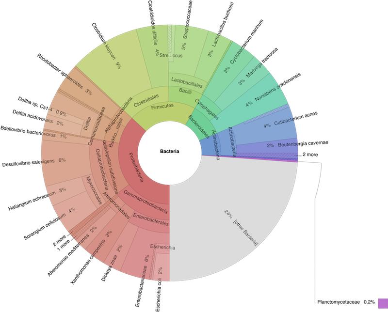
Fig. 6.2 Example of an Krona output webpage.
6.6.1. Installation
Install Krona with:
$ conda create --yes -n krona krona
$ conda activate krona
First some house-keeping to make the Krona installation work. Do not worry to much about what is happening here.
# we delete a symbolic link that is not correct
$ rm -rf ~/miniconda3/envs/ngs/opt/krona/taxonomy

# we create a directory in our home where the krona database will live
$ mkdir -p ~/krona/taxonomy

# now we make a symbolic link to that directory
$ ln -s ~/krona/taxonomy ~/miniconda3/envs/ngs/opt/krona/taxonomy
6.6.2. Build the taxonomy
We need to build a taxonomy database for Krona. However, if this fails we will skip this step and just download a pre-build one. Lets first try to build one.
$ ktUpdateTaxonomy.sh ~/krona/taxonomy
Attention
Should this fail we can download a pre-build database on the Downloads page via a browser.
Once you have downloaded the file, follow these steps:
# we unzip the file
$ gzip -d taxonomy.tab.gz

# we move the unzipped file to our taxonomy directory we specified in the step before.
$ mv taxonomy.tab ~/krona/taxonomy
6.6.3. Visualise
Now, we use the tool ktImportTaxonomy from the Krona tools to create the html web-page.
We first need build a two column file (read_id<tab>tax_id) as input to the ktImportTaxonomy tool.
We will do this by cutting the columns out of either the Kraken2 or Centrifuge results:
# Kraken2
$ cd kraken
$ cat evol1.kraken | cut -f 2,3 > evol1.kraken.krona
$ ktImportTaxonomy evol1.kraken.krona
$ firefox taxonomy.krona.html

# Centrifuge
$ cd centrifuge
$ cat evol1-results.txt | cut -f 1,3 > evol1-results.krona
$ ktImportTaxonomy evol1-results.krona
$ firefox taxonomy.krona.html
What happens here is that we extract the second and third column from the Kraken2 results. Afterwards, we input these to the Krona script, and open the resulting web-page in a bowser. Done!
References
- KIM2017
Kim D, Song L, Breitwieser FP, Salzberg SL. Centrifuge: rapid and sensitive classification of metagenomic sequences. Genome Res. 2016 Dec;26(12):1721-1729
- LU2017
Lu J, Breitwieser FP, Thielen P, Salzberg SL. Bracken: estimating species abundance in metagenomics data. PeerJ Computer Science, 2017, 3:e104, doi:10.7717/peerj-cs.104
- ONDOV2011
Ondov BD, Bergman NH, and Phillippy AM. Interactive metagenomic visualization in a Web browser. BMC Bioinformatics, 2011, 12(1):385.
- WOOD2014
Wood DE and Steven L Salzberg SL. Kraken: ultrafast metagenomic sequence classification using exact alignments. Genome Biology, 2014, 15:R46. DOI: 10.1186/gb-2014-15-3-r46.